Example usage

Version check

import matplotlib.pyplot as plt
import numpy as np

import fbench
from fbench.viz import FunctionPlotter, VizConfig

print(fbench.__version__)

1.0.1

FunctionPlotter

Functions with 1-vector input

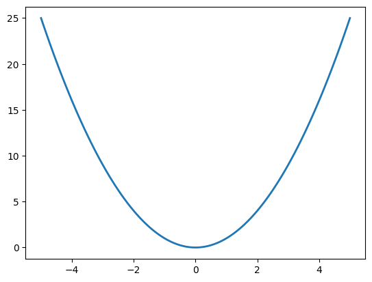
func = lambda x: (x**2).sum()
bounds = [(-5, 5)]

default = FunctionPlotter(func, bounds)
default.plot()
plt.show()

less_grid_points = FunctionPlotter(func, bounds, n_grid_points=7)
less_grid_points.plot()
plt.show()

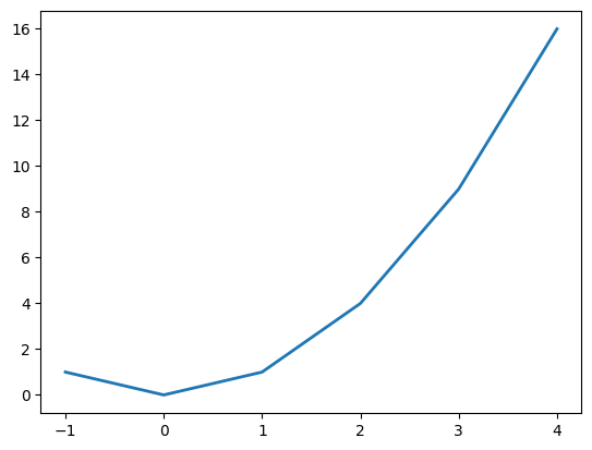
specific_grid_points = FunctionPlotter(
    func,
    bounds,
    x_coord=[-1, 0, 1, 2, 3, 4],
)
specific_grid_points.plot()
plt.show()

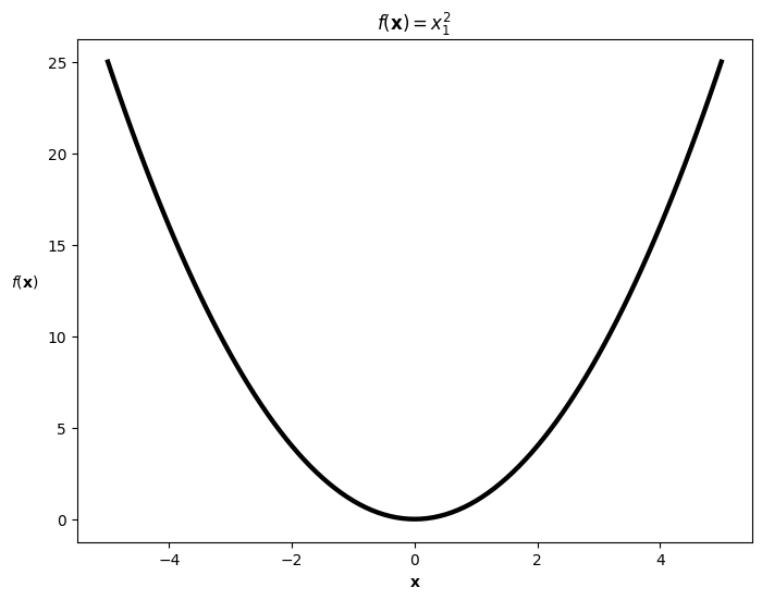
kws_plot = VizConfig.get_kws_plot__base()

kws_plot.update({"color": "black", "linewidth": 3.14159})

custom_kws = FunctionPlotter(
    func,
    bounds,
    kws_plot=kws_plot,
)

_, ax = plt.subplots(1, 1, figsize=(8, 6))

_, ax, _ = custom_kws.plot(ax=ax)

ax.set_xlabel(r"$ \mathbf{x} $")
ax.set_ylabel(r"$ f(\mathbf{x}) $", rotation=0, labelpad=15)
ax.set_title(r"$ f(\mathbf{x}) = x_{1}^{2} $")

plt.show()

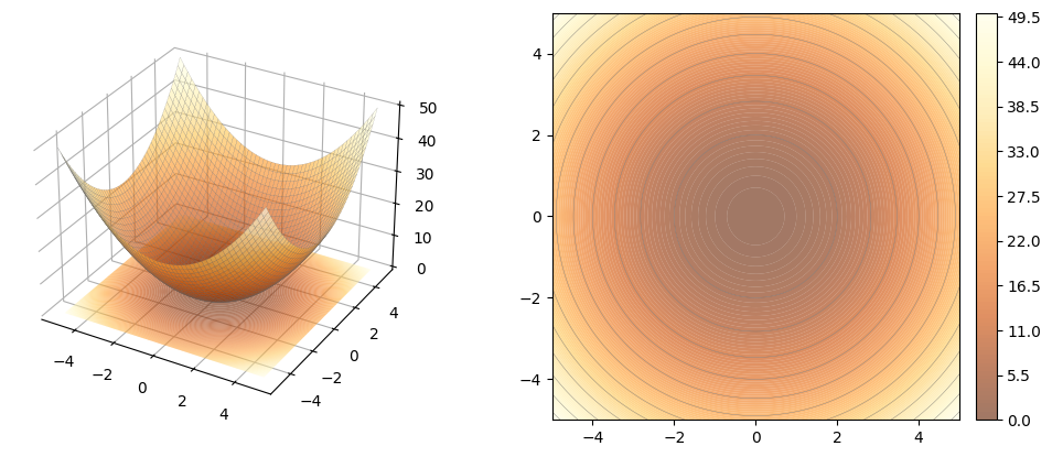
Functions with 2-vector input

func = lambda x: (x**2).sum()
bounds = [(-5, 5)] * 2

default = FunctionPlotter(func, bounds)
default.plot()
plt.show()

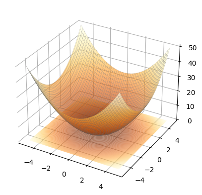
only_surface = FunctionPlotter(func, bounds, with_contour=False)
only_surface.plot()
plt.show()

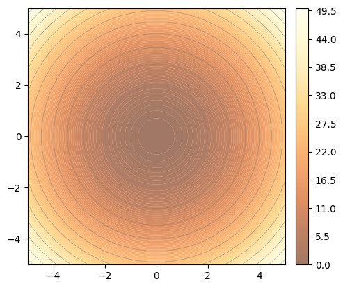
only_contour = FunctionPlotter(func, bounds, with_surface=False)
only_contour.plot()
plt.show()

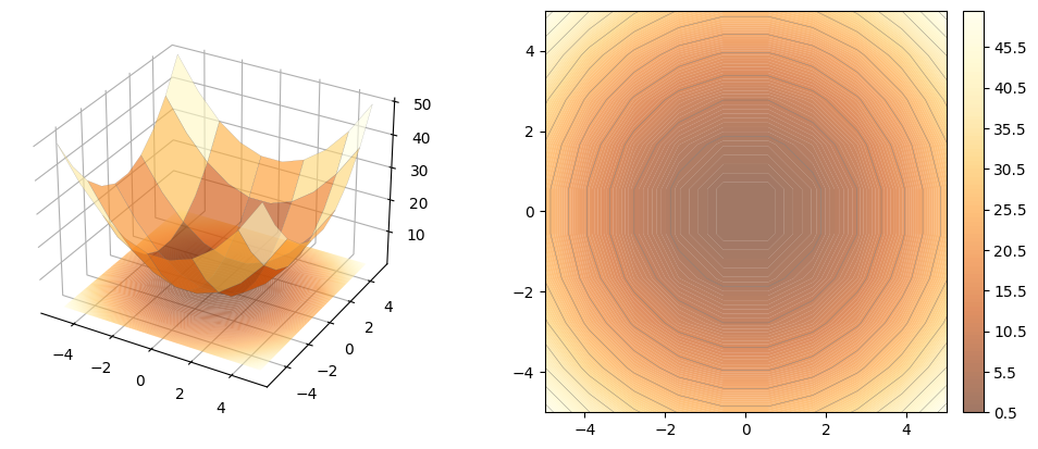
less_grid_points = FunctionPlotter(func, bounds, n_grid_points=10)
less_grid_points.plot()
plt.show()

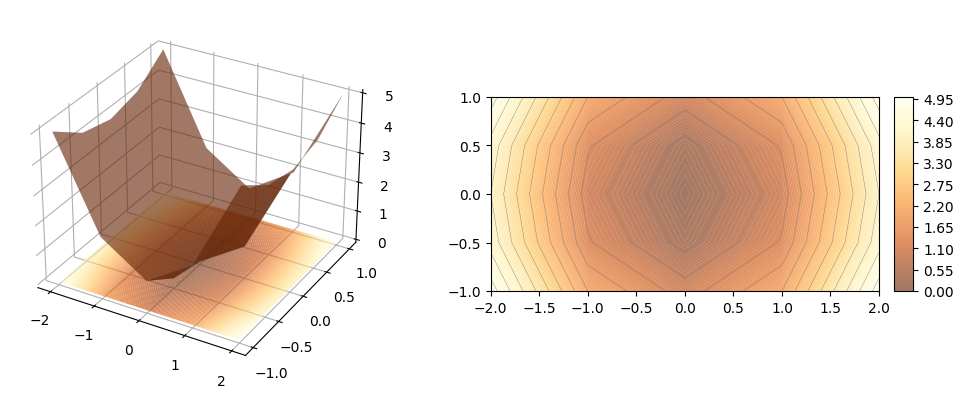
specific_grid_points = FunctionPlotter(
    func,
    bounds,
    x_coord=[-2, -1, 0, 1, 2],
    y_coord=[-1, -0.5, 0, 0.5, 1],
)
specific_grid_points.plot()
plt.show()

plt.colormaps()[::2][:5]

['magma', 'plasma', 'cividis', 'twilight_shifted', 'Blues']

kws_surface = VizConfig.get_kws_surface__base()
kws_contourf = VizConfig.get_kws_contourf__base()
kws_contour = VizConfig.get_kws_contour__base()

kws_surface.update({"cmap": plt.get_cmap("cividis_r")})
kws_contourf.update({"cmap": plt.get_cmap("cividis_r")})
kws_contour.update({"colors": "black", "alpha": 0.4, "levels": 6, "linewidths": 0.414})

custom_kws = FunctionPlotter(
    func,
    bounds,
    kws_surface=kws_surface,
    kws_contourf=kws_contourf,
    kws_contour=kws_contour,
)

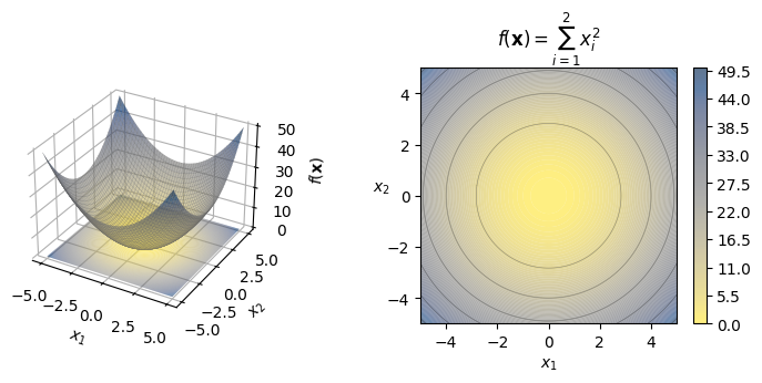
fig = plt.figure(figsize=(9, 3))

_, ax, ax3d = custom_kws.plot(fig=fig)

ax.set_xlabel(r"$ x_{1} $")
ax.set_ylabel(r"$ x_{2} $", rotation=0)
ax.set_title(r"$ f(\mathbf{x}) = \sum_{i=1}^{2} x_i^2 $")

ax3d.set_xlabel(r"$ x_{1} $")
ax3d.set_ylabel(r"$ x_{2} $")
ax3d.set_zlabel(r"$ f(\mathbf{x}) $")

plt.show()

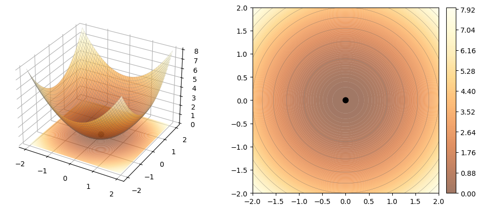
default_with_predefined_func = FunctionPlotter(
    func=fbench.sphere,
    bounds=((-2, 2), (-2, 2)),
)
default_with_predefined_func.plot()
plt.show()

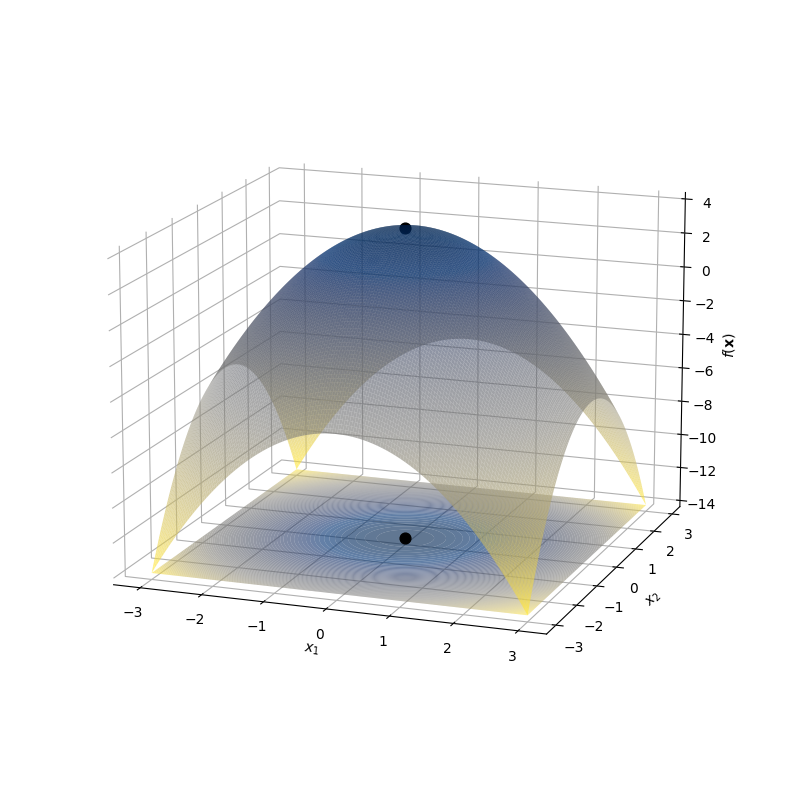
lambda_func_with_manual_optimum = FunctionPlotter(
    func=lambda x: -fbench.sphere(x) + 4,
    bounds=((-3, 3), (-3, 3)),
    with_optima=True,
    optima=[fbench.structure.Optimum(np.zeros(2), 4)],
)
lambda_func_with_manual_optimum.plot()
plt.show()

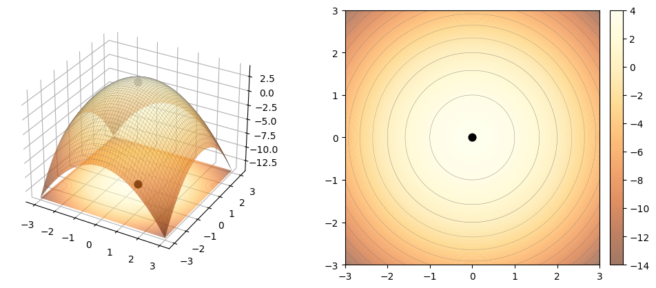
fig = plt.figure(figsize=(24, 10))

kws_surface = dict(cmap=plt.get_cmap("cividis_r"), linewidth=0)
kws_contourf = dict(cmap=plt.get_cmap("cividis_r"))
kws_contour = dict(linewidths=0)

rotated_surface = FunctionPlotter(
    func=lambda x: -fbench.sphere(x) + 4,
    bounds=((-3, 3), (-3, 3)),
    n_grid_points=303,
    with_optima=True,
    optima=[fbench.structure.Optimum(np.zeros(2), 4)],
    with_contour=False,
    kws_surface=kws_surface,
    kws_contourf=kws_contourf,
    kws_contour=kws_contour,
)
_, _, ax3d = rotated_surface.plot(fig=fig)

ax3d.set_xlabel(r"$ x_{1} $")
ax3d.set_ylabel(r"$ x_{2} $")
ax3d.set_zlabel(r"$ f(\mathbf{x}) $")

ax3d.view_init(15, -70, 0)
ax3d.set_box_aspect(None, zoom=0.9)

plt.show()